
Behind AI #5: Machine Learning Algorithms Any AI Enthusiast Should Know - Part 2
Machine learning algorithms explained in plain English


In this second part, we will continue exploring how some algorithms used in Machine Learning work. As we discussed in the first part, there are both supervised and unsupervised algorithms.
Let’s see 6 more algorithms you should know.
1.K-Nearest Neighbors (kNN)
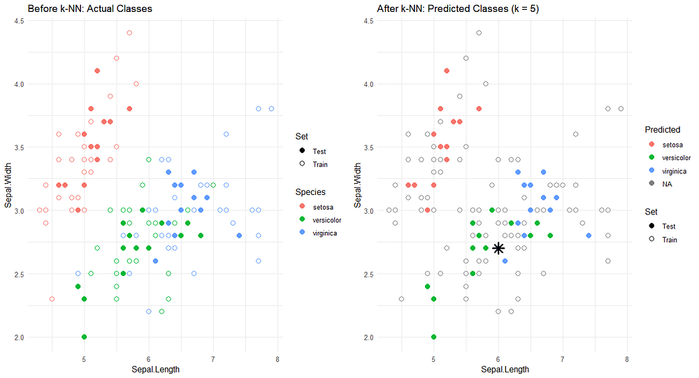
KNN algorithm is a supervised learning technique used for both classification and regression. It’s a simple yet practical method for making predictions. The goal is to find the "k" nearest observations in the feature space and make a decision based on the labels of these neighbors.
Let's break down the key concepts to get a better understanding of how this algorithm works:
The value of "k" is an integer that defines how many neighboring points will be considered.
Distance: To measure how close two points are, a distance metric is usually used. The most common is Euclidean distance, though others like Manhattan, Minkowski, and more can also be applied.
If we use it for classification, the new point is assigned to the most common class among its "k" neighbors (majority voting). If there is a tie, it can be resolved using additional criteria, such as weighting the distances.
If we use it for regression, the prediction is made by averaging the values of the neighbors.
Here’s a representation of how the algorithm performs a classification with a hyperparameter of k = 5.
The advantage of this algorithm is that it’s easy to interpret and implement. Additionally, it doesn't make assumptions about the data distribution. However, it’s important to consider the characteristics of the data since this algorithm is distance-based. Another point to keep in mind is its high computational cost for large datasets. It’s also very sensitive to noise or outliers when k is small, while a very large k can overly smooth the decision.
2. Gradient Boosted Decision Trees (GBDT)
GBDT is a supervised learning algorithm used for both classification and regression tasks. It’s a boosting technique that sequentially combines multiple decision trees, with each tree trying to correct the errors of the one before it. The idea is to add weak models (trees) together to build a more robust model.
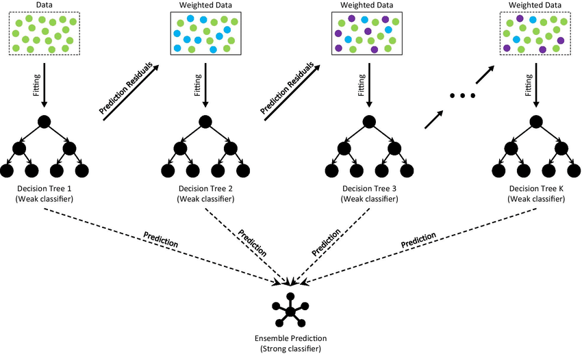
The goal is to minimize error by combining several weak models (decision trees) into a strong model. For regression tasks, the loss function often uses Mean Squared Error (MSE), while for classification, it uses Log-loss.
One of the advantages of GBDT is its strong performance in both classification and regression tasks. It is also a robust model when dealing with outliers, thanks to its ability to handle non-linear data. However, a drawback is that since it uses boosting by adding more trees, the training process can be slower compared to other algorithms. Here, we face the trade-off between performance and speed.
3. K-Means Clustering
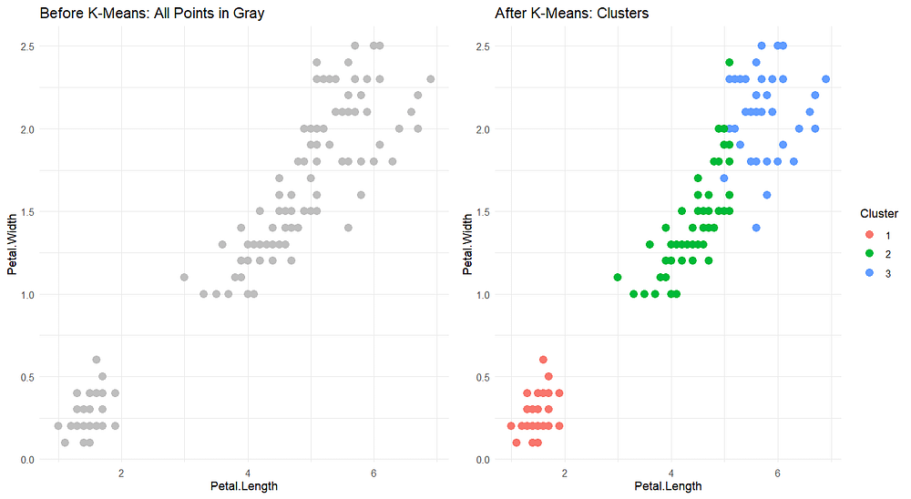
K-Means is an unsupervised clustering algorithm that groups data into k clusters based on their features. The goal is to minimize the distances between the points within a cluster and its centroid, aiming to reduce internal variance. This is an iterative process that essentially forms groups of data points with similar characteristics, distinguishing them from other, more distant groups.
Let’s break down how this algorithm works:
Initialization: Randomly select k centroids, which represent the centers of the initial clusters.
Assign Points to Clusters: Assign each data point to the cluster whose centroid is closest (using Euclidean distance).
Recalculate Centroids: Once all points are assigned, recalculate the centroids of each cluster as the mean of all points within that cluster.
Reassign Points: Reassign each data point to the cluster with the nearest updated centroid.
Repeat: Repeat steps 3 and 4 until the centroids no longer change significantly (or until a maximum number of iterations is reached).
Final Clusters: The data points will then be organized into k clusters, with their respective centroids stabilized.
Now, let’s see how we can use this algorithm to perform the following classification:
4. Hierarchical Clustering
Hierarchical clustering creates a tree-like structure (dendrogram) to group the data. Clusters are formed by either merging (agglomerative) or splitting (divisive) the data iteratively. The goal is to create a hierarchy of clusters that allows data to be grouped at different levels of similarity.
Here’s a step-by-step breakdown of how this algorithm works:
Initialization: Each data point starts as its own individual cluster.
Calculate Distances: Calculate the distances between all clusters, typically using Euclidean distance.
Merge Clusters: In each iteration, merge the two closest clusters (those with the smallest distance).
Update Distances: After merging two clusters, recalculate the distances between the newly formed cluster and the remaining clusters.
Build the Dendrogram: As clusters are merged, the dendrogram visually represents how clusters are combined at each level. The nodes in the tree indicate cluster merges at different heights.
Determine Final Clusters: The final number of clusters can be set by "cutting" the dendrogram at a certain level, corresponding to the desired number of clusters.
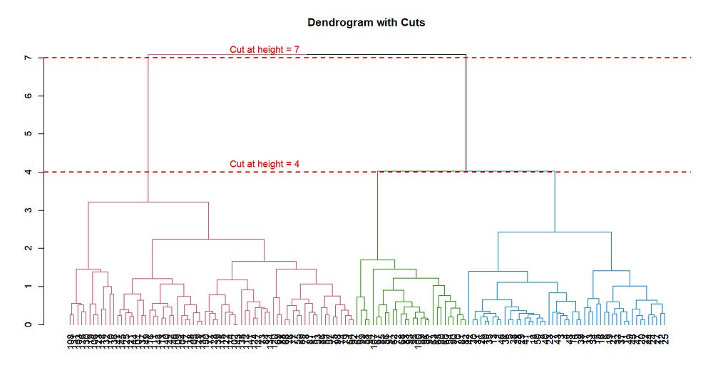
This will lead us to the final result:
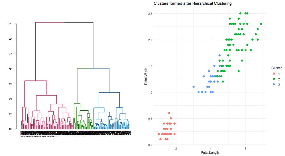
Hierarchical clustering always produces the same clusters. In contrast, K-Means clustering can yield different clusters depending on the initial placement of the centroids (cluster centers). However, hierarchical clustering is slower compared to K-Means. It takes a significant amount of time to run, especially with large datasets.
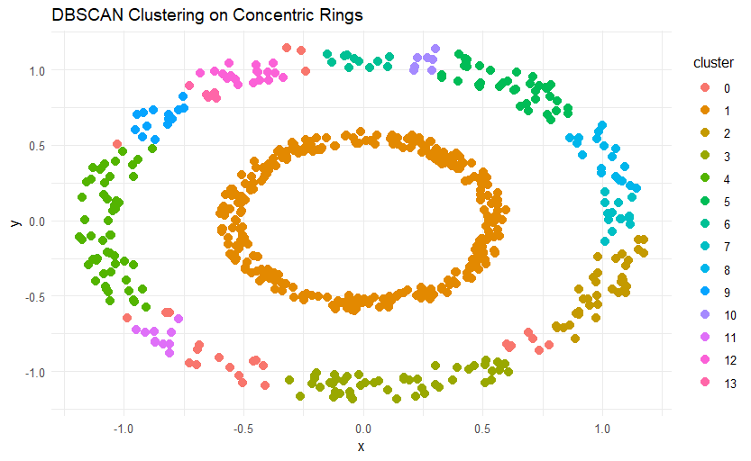
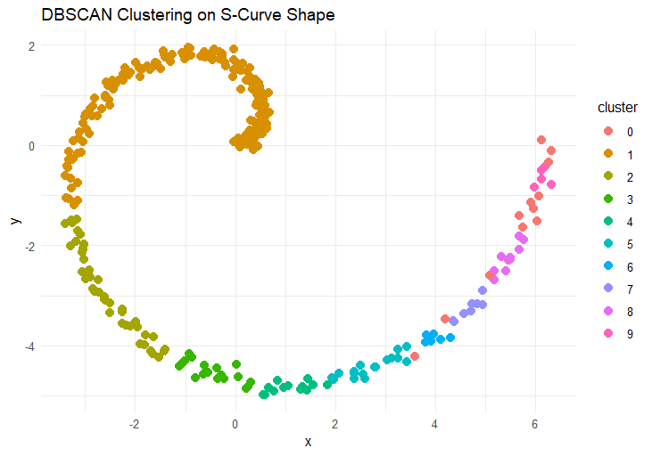
5. DBSCAN Clustering
DBSCAN is a density-based clustering algorithm that groups nearby points and labels isolated points as "noise" or outliers. Unlike K-Means, it does not require you to define the number of clusters in advance. The goal is to identify high-density clusters and mark isolated points.
Here’s a closer look at how this algorithm works:
Parameter Definition: Two key parameters are set: ε (epsilon), which is the radius of the neighborhood around a point, and minPts, the minimum number of points needed to form a cluster.
Initialization: A random point is selected from the dataset.
Neighborhood Density: If there are at least minPts within the ε radius around the selected point, it is considered a core point, and a cluster is formed. If not, the point is marked as noise.
Cluster Expansion: The cluster expands by searching for all points within the ε radius of the points already included in the cluster. If any of these points also have at least minPts neighbors within their ε radius, the cluster continues to grow.
Repeat: This process repeats for each unvisited point. Points that do not meet the density criteria are marked as noise and are not included in any cluster.
Final Clusters: The algorithm concludes by forming clusters of densely packed points, while isolated points are labeled as noise.
In some cases, finding an appropriate neighborhood distance (ε) can be challenging and may require domain expertise.
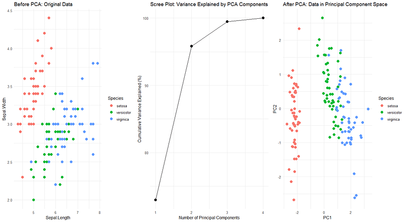
6. Principal Component Analysis (PCA)
PCA is a dimensionality reduction technique used to transform a dataset with many features (variables) into a new set of uncorrelated variables called principal components. These components capture most of the variability in the original data while using the fewest possible dimensions.
Principal components are linear combinations of the original variables that capture the maximum variance in the data. They are calculated by finding the eigenvectors and eigenvalues, which define the direction of the components and indicate how much variance each component explains.
Here is a graphical representation before applying the PCA algorithm. After applying PCA, we select 2 components, as they account for the most explained variance. Finally, we project the original data onto these first 2 components.
One advantage of dimensionality reduction is that it simplifies the visualization and analysis of complex data by reducing the number of dimensions. It also eliminates multicollinearity since using linear combinations of the original variables removes correlations between them. However, a key disadvantage is the loss of interpretability and the sensitivity to variable scaling (if the data is not standardized).