Behind AI #1: Machine Learning Algorithms Any AI Enthusiast Should Know
Machine learning algorithms explained in plain English
Hi!
I created a new series called “AI & Python” which will be focused on learning Python, coding concepts, automation, and creating AI apps. From now on, “Behind AI“ will be focused on what's behind the AI products you love. No programming knowledge will be required. Tech concepts (if any) will be explained in plain English.
Examples of a Behind AI piece are this article and the one you’re reading right now.
P.S. In case you’re not interested in the Python articles, go to settings and turn off notifications for “AI & Python” (leave the rest the same to keep receiving my other emails)
Machine learning (ML) is the field behind all the magic in AI products. If you’re new to ML, you probably must’ve heard of the words “algorithm” or “model” without knowing how they’re related to machine learning.
Here’s a brief explanation in plain English.
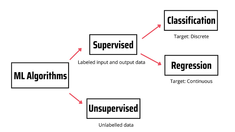
Machine learning algorithms are categorized as supervised or unsupervised. Supervised learning algorithms model the relationship between labeled input and output data (aka target). This model is then used to predict the label of new observations using new labeled input data. If the target variable is discrete, we’re dealing with a classification problem, while if the target variable is continuous we’re dealing with a regression problem. In contrast, unsupervised learning doesn’t rely on labeled input/output data but processes unlabeled data.
Here are 6 supervised learning algorithms that you should know.
1. Linear Regression
Linear regression is the simplest algorithm used in machine learning. This algorithm is used for modeling the relationship between two or more variables. There are two types of linear regression — simple and multiple linear regression.
In simple linear regression, there’s one independent variable and one dependent variable, while in multiple linear regression there are multiple independent variables and one dependent variable.
Here’s the multiple linear regression equation:
where y is the dependent variable (target value), x1, x2, … xn the independent variables (predictors), b0 the intercept, b1, b2, ... bn the coefficients and n the number of observations.
In the picture below, you’ll see a simplified version of the linear regression equation.
As you can see in the picture above, there’s a linear relationship, so if one variable increases or decreases, the other variable will also increase or decrease.
We can use linear regression to predict scores, salaries, house prices, etc. That said, the prediction accuracy isn’t as good as those you’d get with other algorithms.
2. SVM
A Support Vector Machine (SVM) is a supervised learning algorithm that is mostly used in classification problems. We usually feed the SVM model with labeled training data to categorize new text.
SVM is a good choice when we have a limited number of samples and speed is a priority. This is why it’s used when we work with a dataset that has a few thousand of tagged samples in text classification.
To understand much better how SVM works let’s see an example.
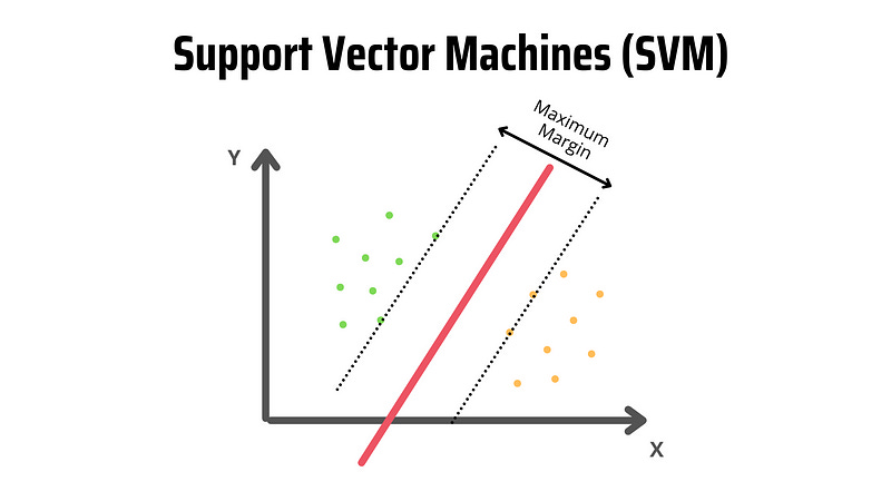
In the picture below, we have two tags (green and yellow) and two features (x and y). Say we want to build a classifier that finds whether our text data is either green or yellow. If that’s the case, we will plot each observation (aka data point) in an n-dimensional space, where “n” is the number of features used.
We only have two features, so the observations are plotted in 2-dimensional space as shown in the picture below.
SVM takes the data points and makes a hyperplane that best separates the classes. Since the observations are plotted in 2-dimensional space, the hyperplane is a line.
This red line is also known as the decision boundary. The decision boundary determines whether a data point belongs to one class or to another. In our example, if the data point falls on the left side, it will be classified as green, while if it falls on the right side, it will be classified as yellow.
3. Decision Tree
If you know nothing about machine learning, you might still know about decision trees.
A decision tree is a model used in planning, statistics, and machine learning that uses a tree-like structure of decisions/consequences to evaluate the possible events involved in a particular problem.
Here’s a decision tree that evaluates scenarios where people want to play football.

Each square is called a node. The last nodes of the decision tree are called the leaves of the tree. To make predictions we start from the root of the tree (first node). Each node in the decision tree will be evaluated. Then we follow the branch that agrees with the evaluation and jump to the next node.
The decision tree algorithm can be used for solving both regression and classification problems. We use a decision tree to build a model that can predict the class or value of the target variable by learning decision tree rules inferred from the training data.
4. Random Forest
Random forest is an ensemble of many decision trees. It combines the simplicity of a decision tree with flexibility resulting in an improvement in accuracy.
To make a random forest, first, we need to create a “bootstrapped” dataset. Bootstrapping is randomly selecting samples from original data (we can even choose the same sample more than once). Then, we use the bootstrapped dataset to create a decision tree.
This method is known as “bagging.” If we repeat the previous steps multiple times, we get a good number of trees. This variety of trees is what makes random forests more effective than a single decision tree.
If the random forest is used for a classification task, the model selects the mode of the predictions of each decision tree. For a regression task, the model selects the mean value of the results from the decision trees.
5. Naive Bayes
Naive Bayes is a supervised learning algorithm that uses conditional probability to predict a class.
The Naive Bayes algorithm is based on the Bayes theorem:
p(A|B): Probability of event A given event B has already occurred
p(B|A): Probability of event B given event A has already occurred
p(A): Probability of event A
p(B): Probability of event B
Naive Bayes assumes that every feature is independent of each other, which isn’t always the case, so we should examine our data before choosing this algorithm.
The assumption that features are independent of each other makes Naive Bayes fast compared to more complex algorithms; however, it also makes this algorithm less accurate.
We can use Naive Bayes to predict weather forecasting, fraud detection, and more.
6. Logistic Regression
Logistic regression is a supervised learning algorithm that is commonly used for binary classification problems. This means we can use logistic regression to predict whether a customer will churn or not, and to find whether a mail is spam or not.
The logistic regression is based on the logistic function (aka the sigmoid function), which takes in a value and assigns a probability between 0 and 1.
Here’s the graph of the logistic regression:
To understand much better how Logistic Regression works, consider a scenario where we need to classify whether an email is spam or not.
In the graph, if Z goes to infinity, Y (our target value) will become 1, which means the email is spam. However, if Z goes to negative infinity, Y will become 0, which means the email is not spam.
The output value is a probability, so if we obtain a value of 0.64, this means that there’s a 64% chance that an email will be spam.
That’s it for now! Let me know in the comments if you want a 2nd part of this.


Great introduction to some essential machine learning algorithms. Looking forward to the 2nd part!
excellent summary! welcome a 2nd part