
Behind AI #4: What is NLP And Why is Important in AI
This is what makes chatbots possible.


Natural language processing (NLP) is a subfield of AI that uses machine learning to enable computers to understand and communicate with human language. NLP is used in various AI applications like chabots.
Today, we’ll learn some common NLP techniques. We’ll focus on the concepts. That said, I added some lines of Python code to better understand the techniques with examples (you don’t need to know coding to understand the examples though).
Natural Language Processing (NLP) is focused on enabling computers to understand and process human language. Computers are great at working with structured data like spreadsheets; however, a lot of the data we generate is unstructured.
We can implement many NLP techniques with just a few lines of Python code thanks to open-source libraries such as spaCy and NLTK. In this article, we’ll dive into the world of NLP by learning some common techniques.
Table of Contents
1. Sentiment Analysis
2. Named Entity Recognition (NER)
3. Stemming
4. Lemmatization
5. Bag of Words (BoW)
6. Term Frequency–Inverse Document Frequency (TF-IDF)
7. Bonus: Wordcloud1. Sentiment Analysis
Sentiment Analysis is a popular NLP technique that involves taking a piece of text (e.g., a comment, review, or a document) and determining whether it’s positive, negative, or neutral. It has many applications in healthcare, customer service, banking, etc.
Python Implementation
For simple cases, in Python, we can use VADER (Valence Aware Dictionary for Sentiment Reasoning) which is available in the NLTK package and can be applied directly to unlabeled text data.
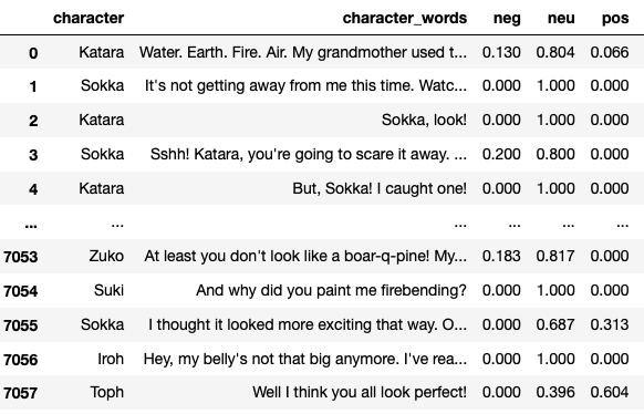
As an example, let’s get all sentiment scores of the lines spoken by characters in a TV show. First, we wrangle a dataset available on Kaggle named ‘avatar.csv’, and then with VADER we calculate the score of each line spoken. All of this is stored in the df_character_sentiment dataframe.
import pandas as pd
import nltk
from nltk.sentiment.vader import SentimentIntensityAnalyzer

# reading and wragling data
df_avatar = pd.read_csv('avatar.csv', engine='python')
df_avatar_lines = df_avatar.groupby('character').count()
df_avatar_lines = df_avatar_lines.sort_values(by=['character_words'], ascending=False)[:10]
top_character_names = df_avatar_lines.index.values

# filtering out non-top characters
df_character_sentiment = df_avatar[df_avatar['character'].isin(top_character_names)]
df_character_sentiment = df_character_sentiment[['character', 'character_words']]

# calculating sentiment score
sid = SentimentIntensityAnalyzer()
df_character_sentiment.reset_index(inplace=True, drop=True)
df_character_sentiment[['neg', 'neu', 'pos', 'compound']] = df_character_sentiment['character_words'].apply(sid.polarity_scores).apply(pd.Series)
df_character_sentiment
In the df_character_sentiment below, we can see that every sentence receives a negative, neutral, and positive score.
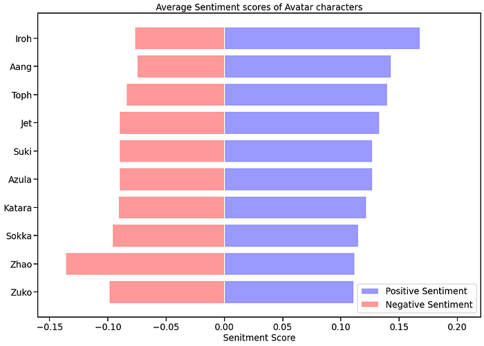
We could group the scores by character and calculate the mean to obtain the sentiment score for a character and then represent it with horizontal bar plots as shown below.
Note: VADER is optimized for social media text, so we should take the results with a grain of salt. You can use a more complete algorithm or develop your own with machine learning libraries. In the link below, there’s a complete guide on how to create one from scratch with Python using the sklearn library.
2. Named Entity Recognition (NER)
Named Entity Recognition is a technique used to locate and classify named entities in text into categories such as persons, organizations, locations, expressions of times, quantities, monetary values, percentages, etc. It‘s used for optimizing search engine algorithms, recommendation systems, customer support, content classification, etc.
Python Implementation
In Python, we can use SpaCy’s named entity recognition that supports the following entity types.
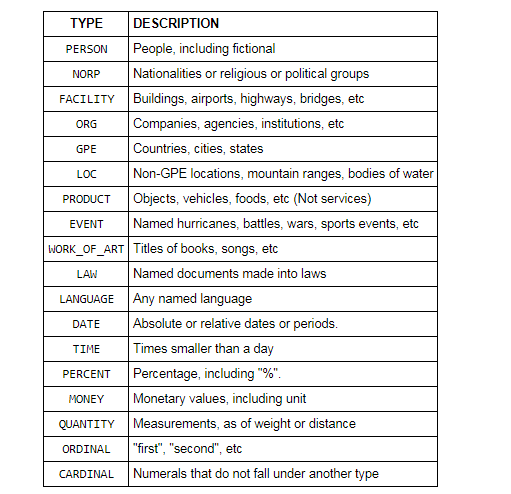
To see it in action, we first import spacy, and then create a nlp variable that will store the en_core_web_sm pipeline. This is a small English pipeline trained on written web text (blogs, news, comments), that includes vocabulary, vectors, syntax, and entities. To find the entities, we apply nlp to a sentence.
Let’s do a test with the following sentence "Biden invites Ukrainian president to White House this summer."
import spacy

nlp = spacy.load("en_core_web_sm")
doc = nlp("Biden invites Ukrainian president to White House this summer")

print([(X.text, X.label_) for X in doc.ents])
Here are the entities we get.
[('Biden', 'PERSON'), ('Ukrainian', 'GPE'), ('White House', 'ORG'), ('this summer', 'DATE')]Spacy found that “Biden” is a person, “Ukranian” is GPE (countries, cities, states, “White House” is an organization, and “this summer” is a date.
3. Stemming & Lemmatization
Stemming and lemmatization are 2 popular techniques in NLP. Both normalize a word but in different ways.
Stemming: It truncates a word to its stem word. For example, the words “friends,” “friendship,” and “friendships” will be reduced to “friend.” Stemming may not give us a dictionary, or grammatical word for a particular set of words.
Lemmatization: Unlike the stemming technique, lemmatization finds the dictionary word instead of truncating the original word. Lemmatization algorithms extract the correct lemma of each word, so they often require a dictionary of the language to be able to categorize each word correctly.
Both techniques are widely used and you should choose them wisely based on your project’s goals. Lemmatization has a lower processing speed, compared to stemming so if accuracy is not the project’s goal but speed, then stemming is an appropriate approach; however. if accuracy is crucial, then consider using lemmatization.
Python’s library NLTK makes it easy to work with both techniques. Let’s see it in action.
Python Implementation (Stemming)
For the English language, there are two popular libraries available in nltk — Porter Stemmer and LancasterStemmer.
from nltk.stem import PorterStemmer
from nltk.stem import LancasterStemmer

# PorterStemmer
porter = PorterStemmer()
# LancasterStemmer
lancaster = LancasterStemmer()

print(porter.stem("friendship"))
print(lancaster.stem("friendship"))
PorterStemmer algorithm doesn’t follow linguistics, but a set of 5 rules for different cases that are applied in phases to generate stems. The print(porter.stem(“friendship”)) code will print the word friendship
LancasterStemmer is simple, but heavy stemming due to iterations and over-stemming may occur. This causes the stems to be not linguistic, or they may have no meaning. The print(lancaster.stem(“friendship”)) code will print the word friend.
You can try any other word to see how both algorithms differ. In the case of other languages, you can import SnowballStemme from nltk.stem
Python Implementation (Lemmatization)
We’ll use NLTK again, but this time we import WordNetLemmatizer as shown in the code below.
from nltk import WordNetLemmatizer

lemmatizer = WordNetLemmatizer()
words = ['articles', 'friendship', 'studies', 'phones']

for word in words:
    print(lemmatizer.lemmatize(word))
Lemmatization generates different outputs for different Part Of Speech (POS) values. Some of the most common POS values are verb (v), noun (n), adjective (a), and adverb (r). The default POS value in lemmatization is a noun, so the printed values for the previous example will be article, friendship, study and phone.
Let’s change the POS value to verb (v).
from nltk import WordNetLemmatizer

lemmatizer = WordNetLemmatizer()
words = ['be', 'is', 'are', 'were', 'was']

for word in words:
    print(lemmatizer.lemmatize(word, pos='v'))
In this case, Python will print the word be for all the values in the list.
5. Bag of Words
The Bag of Words (BoW) model is a representation that turns text into fixed-length vectors. This helps us represent text into numbers so we can use it for machine learning models. The model doesn’t care about the word order, but it’s only concerned with the frequency of words in the text. It has applications in NLP, information retrieval from documents, and classifications of documents.
The typical BoW workflow involves cleaning raw text, tokenization, building a vocabulary, and generating vectors.
Python Implementation
Python’s library sklearn contains a tool called CountVectorizer that takes care of most of the BoW workflow.
Let’s use the following 2 sentences as examples.
Sentence 1: “I love writing code in Python. I love Python code”
Sentence 2: “I hate writing code in Java. I hate Java code”
Both sentences will be stored in a list named text. Then we’re going to create a dataframe df to store this text list. After this, we‘ll initiate an instance of CountVectorizer(cv), and then we’ll fit and transform the text data to obtain the numeric representation. This will be stored in a document-term matrix df_dtm.
import pandas as pd
from sklearn.feature_extraction.text import CountVectorizer
text = ["I love writing code in Python. I love Python code",
"I hate writing code in Java. I hate Java code"]
df = pd.DataFrame({'review': ['review1', 'review2'], 'text':text})
cv = CountVectorizer(stop_words='english')
cv_matrix = cv.fit_transform(df['text'])
df_dtm = pd.DataFrame(cv_matrix.toarray(),
index=df['review'].values,
columns=cv.get_feature_names())
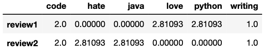
df_dtmThe BoW representation made with CountVectorizer stored in df_dtm looks like the picture below. Keep in mind that words with 2 letters or fewer are not taken into account by the CountVectorizer.
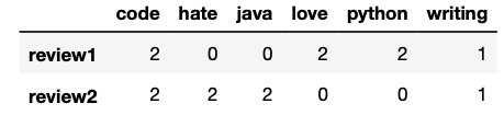
As you can see the numbers inside the matrix represent the number of times each word was mentioned in each review. Words like “love,” “hate,” and “code” have the same frequency (2) in this example.
Overall, we can say that CountVectorizer does a good job tokenizing text, building a vocabulary, and generating vectors.
6. Term Frequency–Inverse Document Frequency (TF-IDF)
Unlike the CountVectorizer, the TF-IDF computes “weights” that represent how relevant a word is to a document in a collection of documents (aka corpus). The TF-IDF value increases proportionally to the number of times a word appears in the document and is offset by the number of documents in the corpus that contain the word. Simply put, the higher the TF-IDF score, the rarer or unique or valuable the term and vice versa. It has applications in information retrieval like search engines that aim to deliver results that are most relevant to what you’re searching for.
Before we see the Python implementation, let’s see an example so you have an idea of how the TF and IDF are calculated. For the following example, we’ll use the same sentences used for the CountVectorizer example.
Sentence 1: “I love writing code in Python. I love Python code”
Sentence 2: “I hate writing code in Java. I hate Java code”
Term Frequency (TF)
There are different ways to define the term frequency. One suggests the raw count itself (i.e., what the Count Vectorizer does), but others suggest it’s the frequency of the word in the sentence divided by the total number of words in the sentence.
For this simple example, we’ll use the first criteria. The term frequency is shown in the following table.
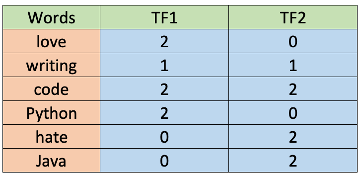
As you can see, the values are the same as the ones calculated for the CountVectorizer before. Also, words with 2 letters or fewer are not taken into account.
Inverse Document Frequency (IDF)
The IDF is also calculated in different ways. Although standard textbook notation defines the IDF as idf(t) = log [ n / (df(t) + 1), the sklearn library we’ll use later in Python calculates the formula by default as follows.
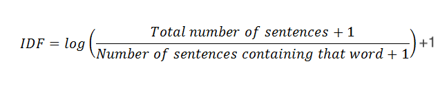
Also, sklearn assumes natural logarithm ln instead of log and smoothing (smooth_idf=True). Let’s calculate the IDF values for each word as sklearn will do it.
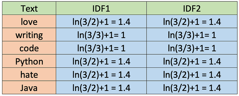
TF-IDF
Once we have the TF and IDF values, we can obtain the TF-IDF by multiplying both values (TF-IDF = TF * IDF). The values are shown in the table below.
Python Implementation
Calculating the TF-IDF shown in the table above in Python requires a few lines of code thanks to the sklearn library.
import pandas as pd
from sklearn.feature_extraction.text import TfidfVectorizer

text = ["I love writing code in Python. I love Python code",
        "I hate writing code in Java. I hate Java code"]

df = pd.DataFrame({'review': ['review1', 'review2'], 'text':text})
tfidf = TfidfVectorizer(stop_words='english', norm=None)
tfidf_matrix = tfidf.fit_transform(df['text'])
df_dtm = pd.DataFrame(tfidf_matrix.toarray(),
                      index=df['review'].values,
                      columns=tfidf.get_feature_names())
df_dtm
The TF-IDF representation stored in df_dtm is presented below.
Note: By default TfidfVectorizer() uses l2 normalization, but to use the same formulas shown above we set
norm=Noneas a parameter. For more details of the formulas used by default in sklearn and how you can customize it check its documentation.
Bonus: Wordcloud
Wordcloud is a popular technique that helps us identify the keywords in a text. It’s not considered as a NLP technique but it still uses some of the techniques explained in this article.
In a wordcloud, more frequent words have a larger and bolder font, while less frequent words have smaller or thinner fonts. In Python, you can make simple wordclouds with the wordcloud library and nice-looking wordclouds with the stylecloudlibrary.
Below you can find the code to make a wordcloud in Python. I’m using a text file of a Steve Jobs speech.
import stylecloud

stylecloud.gen_stylecloud(file_path='SJ-Speech.txt',
                          icon_name= "fas fa-apple-alt")
This is the result of the code above.
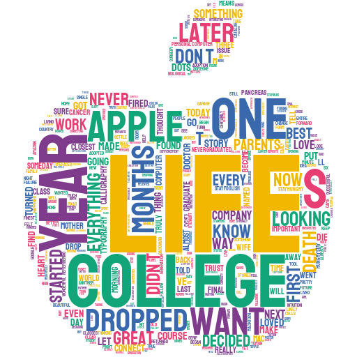
Wordclouds are popular because they’re engaging, easy to understand, and easy to create.
You can take customization even further by changing the colors, removing stopwords, choosing your image, or even adding your own image as a mask of the wordcloud.
what a very nice run-through of getting to grips with NLP. I really enjoyed it.